MIND MELD

Paper: HRI 2022 Citation Github

Motivation and Background

Let’s envision a future where humans and robots are working together out in the real-world, for example, assistive robots in the home. This is a difficult problem because the real-world can be unstructured and unpredictable (e.g., the floor of my house is covered in dog toys that my robot vaccuum regularly gets stuck on). Ideally, robots would be pre-programmed to know how to act in any situation; however, it is impossible for programmers to predict every situation that a robot may encounter. Additionally, people have different preferences and needs. One person might want their cups put away in the cabinet right-side-up, whereas someone else may prefer cups to be upside-down. Therefore, the end-user should be able to communicate their needs and preferences to a robot, without needing programming experience.

One method that enables non-expert users to teach robots new skills is Learning from Demonstration (LfD). With LfD, the person shows the robot how they want the task done, and the robot learns from the person’s demonstration. There are two main types of LfD: Human-centric and Robot-centric LfD. Human-centric LfD is the easiest for humans because the human performs the task, while the robot observes. For example, to teach an autonomous vehicle the correct way to drive, the person would simply drive the car. However, the robot only sees correct examples of how to do the task and does not learn how to recover from mistakes. To solve this problem, in Robot-centric LfD, the robot attempts the task and the human provides corrective feedback to the robot. In the autonomous vehicle example, the vehicle would drive, while the person moves the steering wheel to teach the robot what it should be doing instead. If the robot gets off course, the person can show the robot how to get back on track. The problem with Robot-centric LfD is that people tend to provide suboptimal feedback, due to fatigue, humans not understanding how the robot learns, etc. Incorrect feedback makes it harder for the robot to learn effectively. Also, people provide heterogenous feedback, meaning that people have different teaching strategies. In the autonomous vehicle example, when the robot is making a wrong turn, some demonstrators may turn the wheel all the way in the other direction (over-correcting), whereas others may only turn the wheel a small amount (under-correcting). In this project, we take advantage of the benefits of Robot-centric LfD, and mitigate the problems by creating a method that can learn from suboptimal and heterogenous demonstrators.

Our method is called Mutual Information-driven Meta-learning from Demonstration (MIND MELD) (Schrum et al., 2022).

Overview

MIND MELD works by first using a person’s corrective demonstrations to learn how they are teaching suboptimally. In the driving domain, the person provides demonstrations by moving the steering wheel. In this case, the ways they can be suboptimal are over/under-correcting (moving the steering wheel too much or too little) or being anticipatory/delayed (moving the wheel too early or too late). MIND MELD learns a continous embedding that describes the person’s suboptimal behavior. Then, MIND MELD utilizes this embedding to shift the person’s corrective demonstrations closer to an optimal demonstration.

MIND MELD learns how the person is teaching suboptimally and improves the human's labels.

Optimal Labels and Calibration Tasks

How do we define optimal? In this case, an optimal corrective label steers the car in the shortest path to the goal, while avoiding obstacles.

In order to learn a person’s suboptimal teaching style, we need to compare their corrective labels to optimal labels. Therefore, we calculate optimal labels for a small set of calibration tasks. These calibration tasks are a simple representative subset of tasks. In the driving domain, examples of calibration tasks are the car turning left when it should have gone right or going straight and hitting an obstacle when it should have turned left around the obstacle.

With a more complicated robot task, we envision the person needing to teach the robot a few simple tasks with a block (e.g., pick and place, pushing the block, etc.) to calibrate the robot, meaning the robot learns the person’s suboptimal embedding. Then the person could move on to teaching the robot house cleaning tasks, and the robot could correct for the person’s suboptimal teaching style.

Note: We only need ground truth labels for the calibration tasks. We do not know optimal labels for test tasks.

Network Architecture

The MIND MELD network architecture is in the figure below.

MIND MELD Architecture

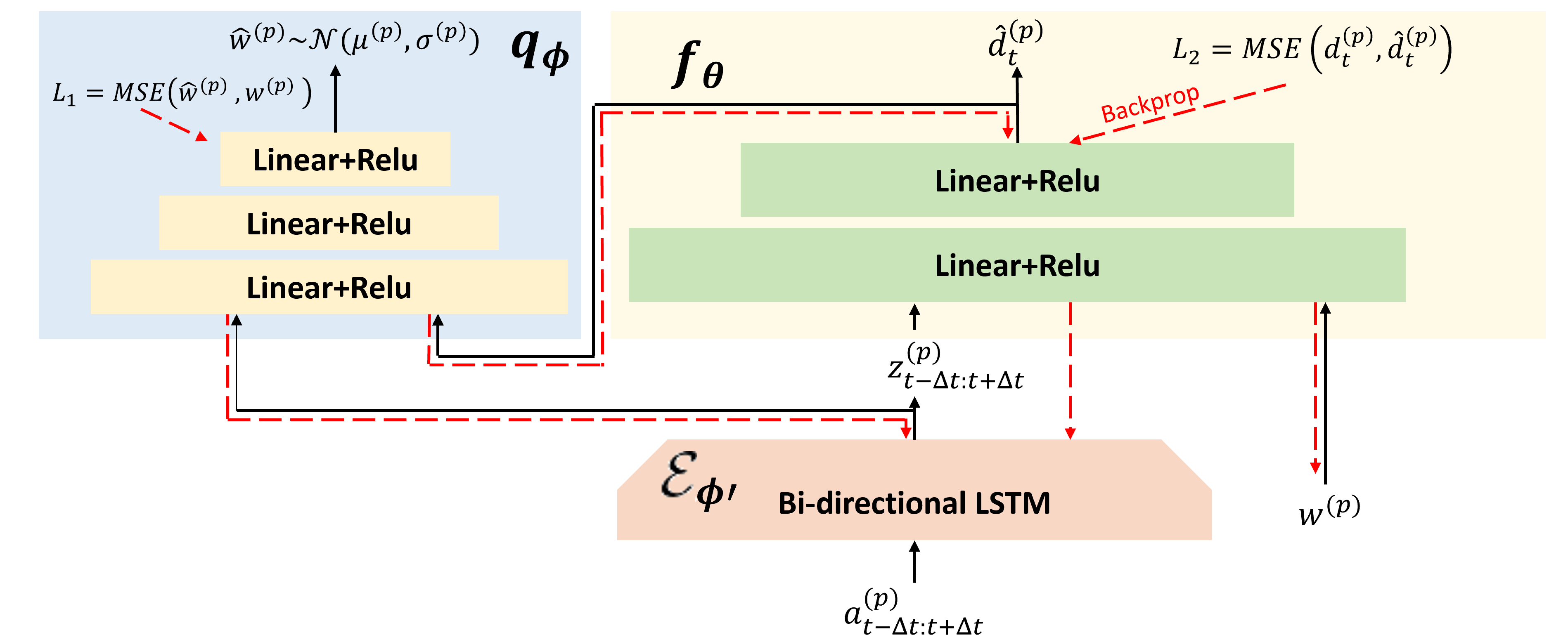
The MIND MELD architecture consists of three parts: 1) the bi-directional Long Short-Term Memory (LSTM) encoder, \(\mathcal{E}_{\phi'}\), 2) the prediction subnetwork, \(f_\theta\), and 3) the recreation subnetwork, \(q_\phi\). The goal of the prediction subnetwork, \(f_\theta\), is to use the demonstrator \(p\)’s corrective feedback, \(a_t^{(p)}\), and the demonstrator’s suboptimal embedding, \(w^{(p)}\), to learn the difference between the demonstrator’s feedback and optimal, \(\hat{d}_{t}^{(p)}\). Additionally, the goal of the recreation subnetwork, \(q_\phi\) is to learn the personalized embedding, \(w^{(p)}\), from the demonstrator labels and how far their labels are from optimal.

Training Phases:

Calibration Phase: A set of users complete the calibration tasks, where we know the ground truth labels. We collect a dataset to learn the MIND MELD parameters, \(\theta, \phi, \phi'\). The parameters are then frozen for the testing phase.
Testing Phase: A new user completes the calibration tasks to determine their personalized embedding, \(w^{(p)}\). Using \(w^{(p)}\), we calculate how much their demonstration should be shifted, \(\hat{d}_{t}^{(p)}\), on a new task (where optimal is unknown).

Bi-directional LSTM, \(\mathcal{E}_{\phi'}\): The input, \(a_t^{(p)}\) is demonstrator \(p\) ‘s corrective label at time \(t\). The \(\Delta t\) labels before and after time \(t\) are passed into the bi-directional LSTM encoder. We use a bi-directional LSTM because the labels are not independent through time, meaning that the labels before and after the current label can provide information about the person’s teaching style. The bi-directional LSTM encodes the timeseries input into an encoding, \(z^{(p)}_{t-\Delta t: t+\Delta t}\).

Prediction Subnetwork, \(f_\theta\) : The encoded demonstrator feedback, \(z^{(p)}_{t-\Delta t: t+\Delta t}\), and the personalized embedding describing the person’s suboptimal teaching style, \(w^{(p)}\), is fed through the prediction subnetwork, \(f_\theta\). The prediction subnetwork then outputs \(\hat{d}_{t}^{(p)}\), which is the amount that the person’s corrective demonstration should be shifted to be closer to optimal. We train this subnetwork using the calibration tasks where we have access to optimal labels, \(o_t\). We utilize a mean-squared error (MSE) loss between the predicted difference, \(\hat{d}_{t}^{(p)}\), and the true difference, \(d_{t}^{(p)}\), where \(d_{t}^{(p)} = a_t^{(p)} - o_t\).

The recreation subnetwork, \(q_\phi\), learns the estimate for the personalized embedding, \(\hat{w}^{(p)}\), and \(w^{(p)}\) is also an input to the architecture. We use the calibration tasks to estimate a user’s embedding, \(\hat{w}^{(p)}\). When we are determining a user’s embedding, we intialize \(w^{(p)}\) to the average embedding from all previous users. The input is updated through backpropagation during each round of training. After the user has completed the calibration tasks and is moving on to teaching the robot a new task, we use the estimated embedding, \(\hat{w}^{(p)}\), as the input.

Recreation Subnetwork, \(q_\phi\) : The recreation subnetwork, \(q_\phi\), takes the encoded demonstrator feedback, \(z^{(p)}_{t-\Delta t: t+\Delta t}\), and the amount that the person is suboptimal, \(\hat{d}_{t}^{(p)}\), to estimate the embedding that describes the person’s suboptimal teaching style, \(\hat{w}^{(p)}\). To estimate \(w^{(p)}\), we utilize variational inference by maximizing the mutual information between \(\hat{d}_{t}^{(p)}\), \(w^{(p)}\), and \(z^{(p)}_{t-\Delta t: t+\Delta t}\). We train this subnetwork using an MSE loss between the estimated embedding, \(\hat{w}^{(p)}\), and the previous guess, \(w^{(p)}\). The intuition here is that the more we learn about how to correct the person’s feedback (as our estimate for \(\hat{d}_{t}^{(p)}\) becomes more accurate), we can be more certain of our estimate for \(w^{(p)}\). Please see the paper for more details and equations.

Experiment and Selected Results

To evaluate MIND MELD, we conduct a human-subjects experiment. In the study, the robot is an autonomous vehicle in a driving simulator, and participants teach the car to drive to a goal location without hitting any obstacles.

Participants teach a car in a driving simulator to drive using a physical steering wheel. The goal is to navigate the car to the large orange ball, without hitting any obstacles.

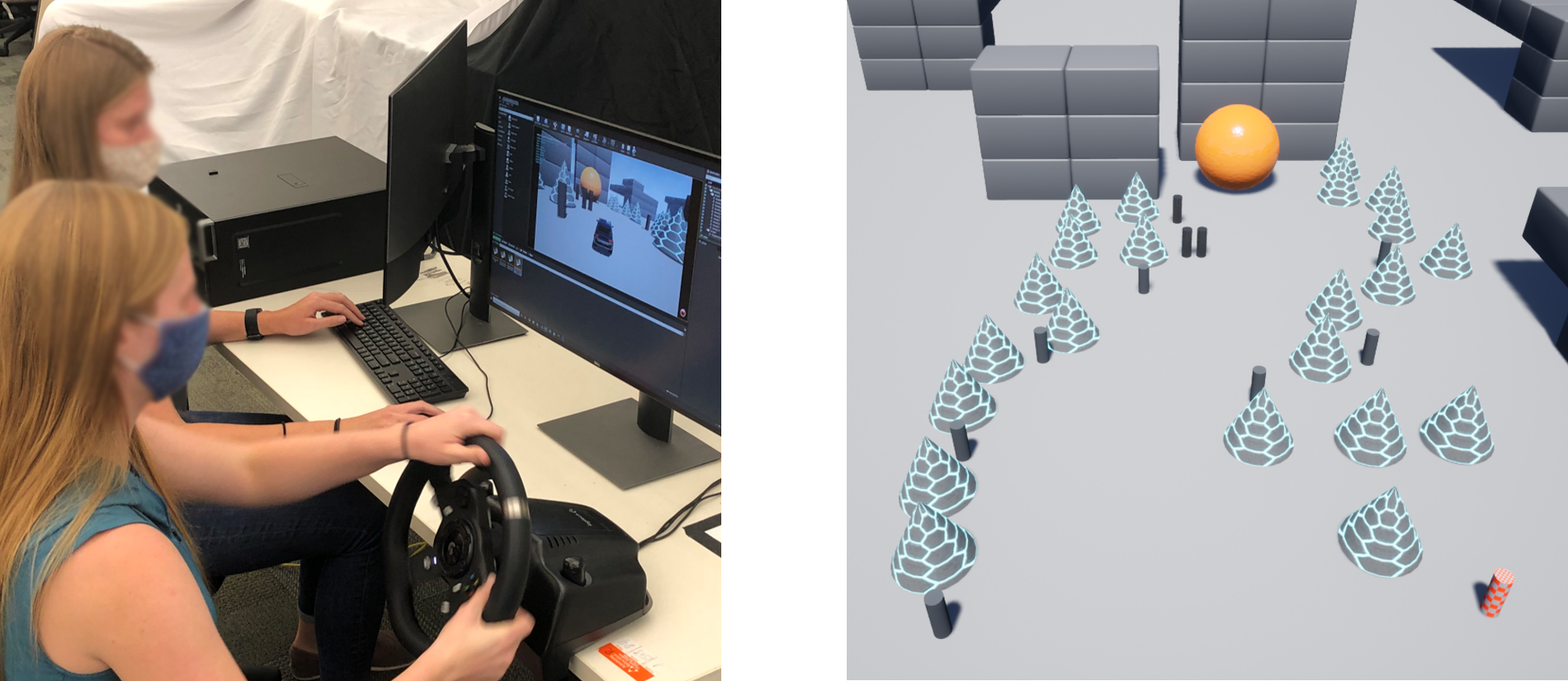
For the Calibration Phase, where we train the MIND MELD architecture parameters, we recruited 76 participants. In this phase, participants completed the calibration tasks, where we have the optimal labels.

To evaluate MIND MELD, we conduct a Testing Phase. In the testing phase, participants first completed the calibration tasks so we could learn their personalized embedding, \(w^{(p)}\). Then participants teach the car to drive on a new, more complicated task (increased number of obstacles and turns needed to reach the goal). Participants teach the car to drive the new task for three different algorithms (in a random order): MIND MELD, a robot-centric baseline (DAgger), and a human-centric baseline (Behavioral Cloning (BC)). For each algorithm, participants teach the car for twelve trials. We recruited 42 participants for this phase.

Metrics

To compare the accuracy of MIND MELD to the baselines, we measure the average distance to the goal and the probability of reaching the goal for each trial. Participants also complete surveys to measure the amount of perceived workload to teach using each algorithm and the likeability, perceived intelligence, and trust of each algorithm.

Overall, we found that MIND MELD outperformed both baselines in terms of accuracy and participant perceptions!

Average Distance from Goal

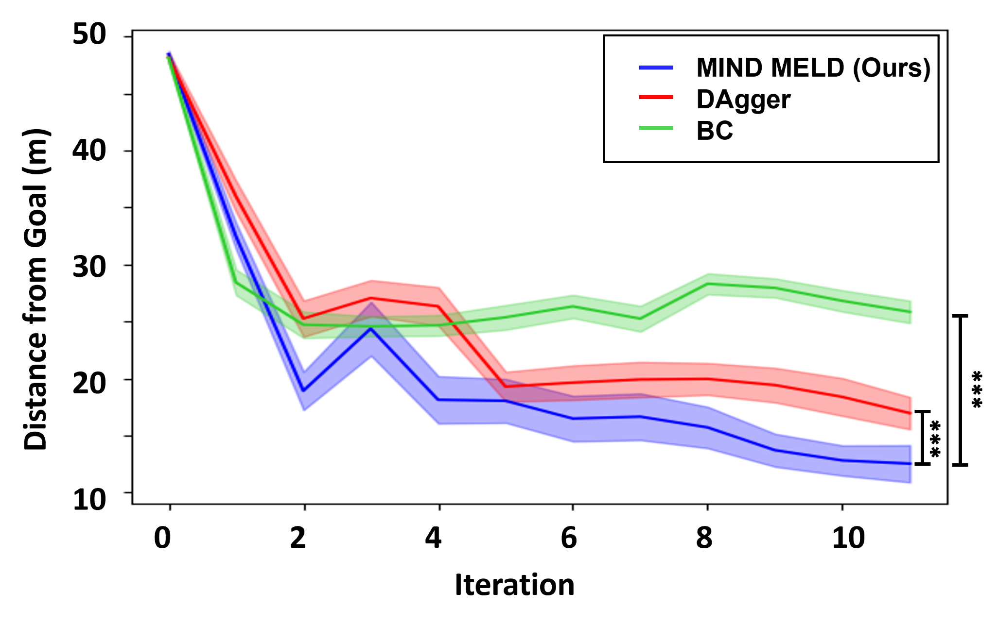
MIND MELD gets significantly closer to the goal compared to both baselines.

Probability of Reaching the Goal

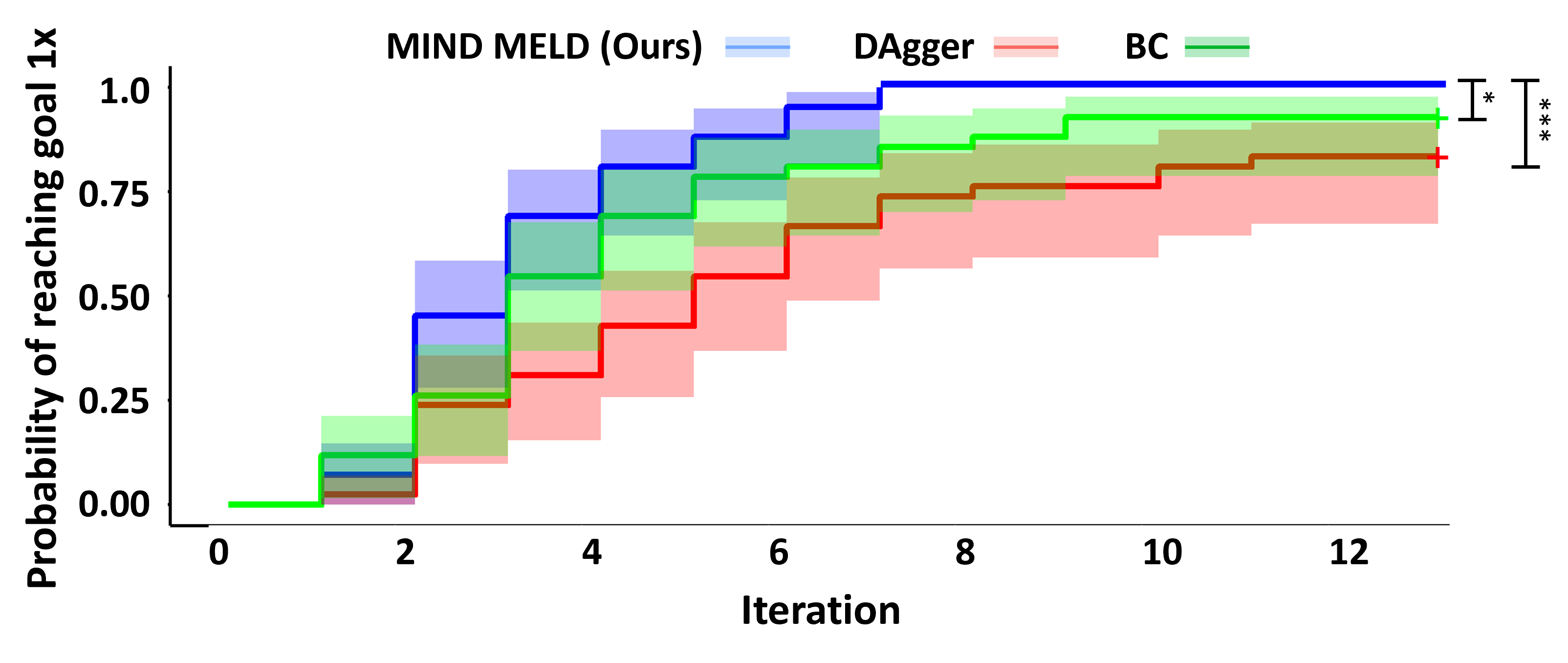
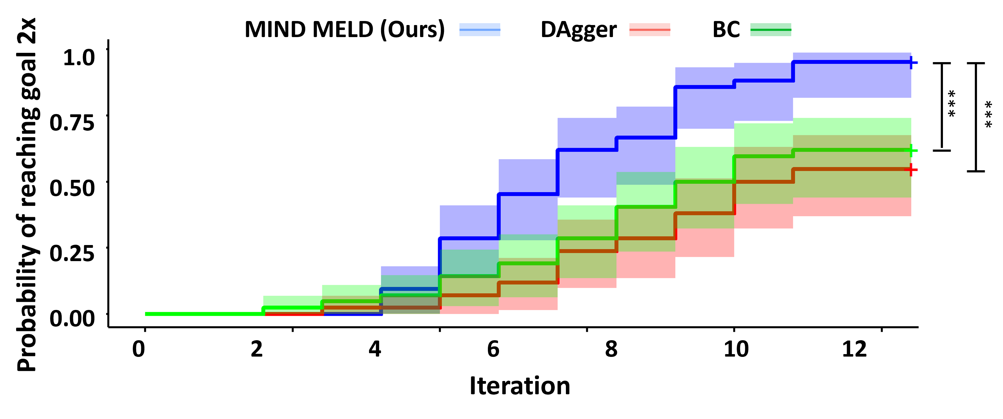
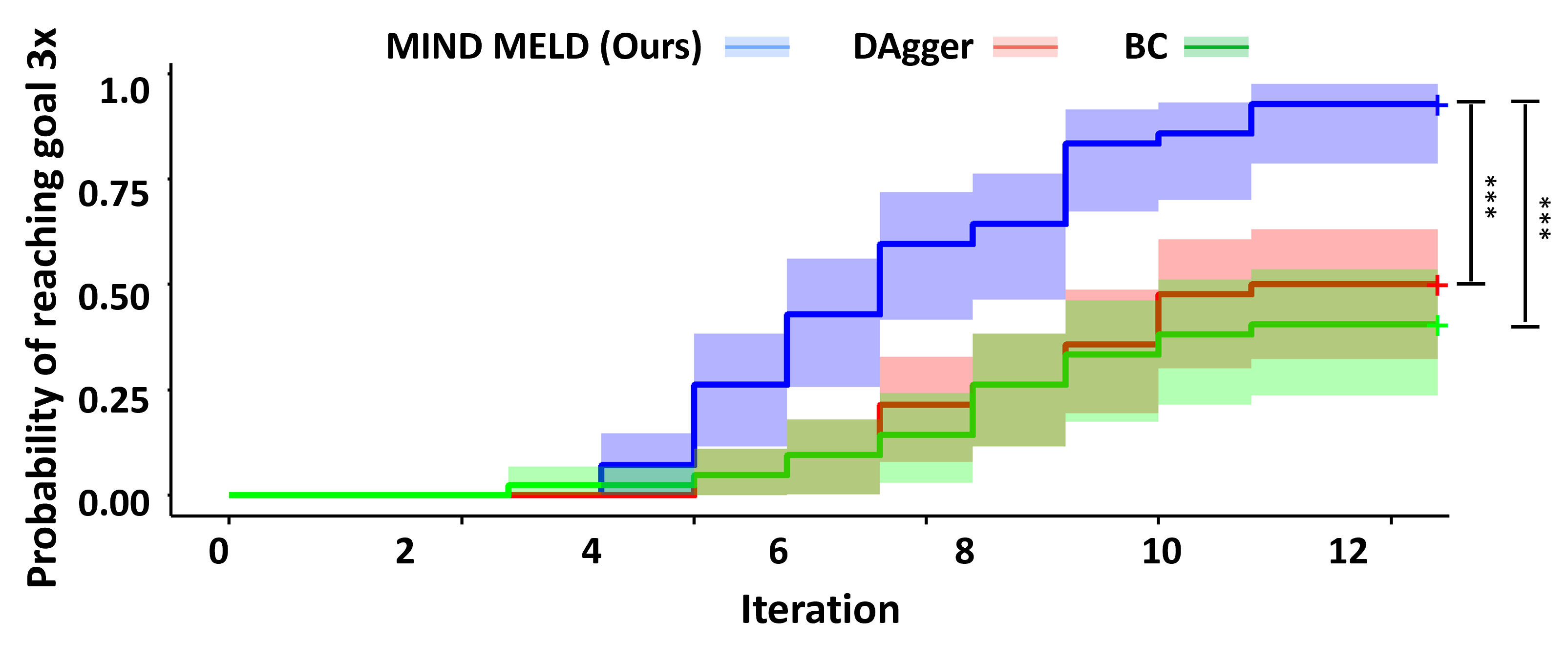
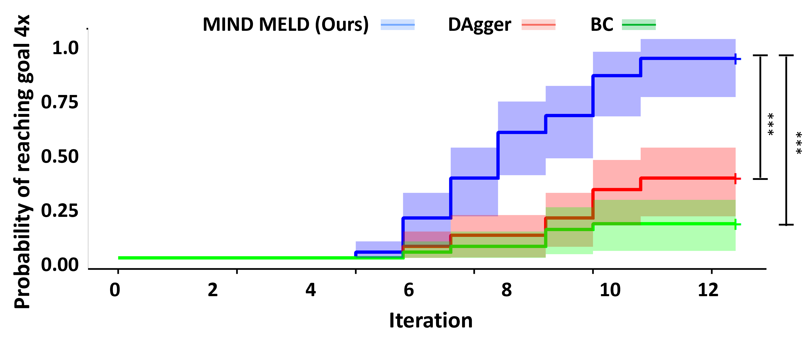
In these plots, we compare the probability of each algorithm reaching the goal once (top left), twice (top right), three times (bottom left), and four times (bottom right) for each trial. Overall, MIND MELD has a significantly higher probability of reaching the goal compared to baselines. In the bottom right plot, MIND MELD has a 100% chance of reaching the goal four times during the trials, while both baselines have less than a 50% chance of achieving the same performance.

Subjective Metrics

Participants rated MIND MELD has significantly less work to teach compared to baselines. Participants also perceived MIND MELD as more likeable and intelligent and trusted MIND MELD more compared to baselines.

Learning from demonstration (LfD) techniques seek to enable users without computer programming experience to teach robots novel tasks. There are generally two types of LfD: human- and robot-centric. While human-centric learning is intuitive, human centric learning suffers from performance degradation due to covariate shift. Robot-centric approaches, such as Dataset Aggregation (DAgger), address covariate shift but can struggle to learn from suboptimal human teachers. To create a more human-aware version of robot-centric LfD, we present Mutual Information-driven Meta-learning from Demonstration (MIND MELD). MIND MELD meta-learns a mapping from suboptimal and heterogeneous human feedback to optimal labels, thereby improving the learning signal for robot-centric LfD. The key to our approach is learning an informative personalized em-bedding using mutual information maximization via variational inference. The embedding then informs a mapping from human provided labels to optimal labels. We evaluate our framework in a human-subjects experiment, demonstrating that our approach improves corrective labels provided by human demonstrators. Our framework outperforms baselines in terms of ability to reach the goal (p<.001), average distance from the goal (p=.006), and various subjective ratings (p=.008).